Statistical Rethinking #

Statistical Rethinking is a textbook by Richard McElreath which builds up the foundations of statistics through thinking about models instead of test, taking an entirely Bayesian approach. These are some notes I made and thoughts I had while reading the book.

Notes #

Julia code #

I am trying to reproduce all the code in the book in Julia as an excuse to learn the language.

2. Small worlds and large worlds #

• 2.1 The Garden of Forking Data

  • 2.1.1-2 Counting possibilities and combining other information

    Gives a nice “garden of forked data” example with a simple blue/white ball setup. Similar to the approach by Gelman at al (Bayesian statistics).

  • 2.1.3 From counts to probability

    In Julia we can use the norm function from the LinearAlgebra package in the standard library to normalise the frequency vector in a vector of “plausibilities”.

    using LinearAlgebra
    x = [0, 3, 8, 9, 0];
    print(x / norm(x, 1))
    

    5-element Vector{Int64}:
     0
     3
     8
     9
     0
    [0.0, 0.15, 0.4, 0.45, 0.0]
    

• 2.2 Building a model

  • 2.2.1 A data story
  • 2.2.2 Bayesian updating
  • 2.2.3 Evaluate

• 2.3 Components of the model

  • 2.3.1 Variables

  • 2.3.2 Definitions

    In Julia let’s build the binomial density function ourselves by implementing the formula at the bottom of page 33,

    \[ P(W, L\mid p) = \frac{(W+L)!}{W!L!}p^W (1-p)^W \]

    using Distributions
    
    function dbinom(n::Integer, size::Integer, prob::Real)
        binomial(size, n) * prob^n * (1.0-prob)^(size-n)
    end;
    
    dbinom( 6, 9, 0.5 )
    

    dbinom (generic function with 1 method)
    0.1640625
    

  • 2.3.3 A model is born

• 2.4 Making the model go

  • 2.4.1 Bayes’ Theorem
  • 2.4.2 Motors

  • 2.4.3 Grid approximation

    Here we will implement the simple Binomial grid approximation example in Julia.

    using Plots
    using Distributions
    
    function dbinom(n::Integer, size::Integer, prob::Real)
        binomial(size, n) * prob^n * (1.0-prob)^(size-n)
    end;
    
    p_grid = collect(0:1/19:1)
    prior = fill(1, 20)
    likelihood = dbinom.( Ref(6), Ref(9), p_grid)
    unstandardised_posterior = likelihood .* prior
    posterior = unstandardised_posterior / sum(unstandardised_posterior)
    f = plot(p_grid,
    	 posterior,
    	 markershape = :circle,
    	 xlabel="probability of water",
    	 ylabel="posterior probability",
    	 title="20 points",
    	 color=:black,
    	 legend=false)
    savefig(f, "~/roam/img/rethinking_stats_2_4_3.png")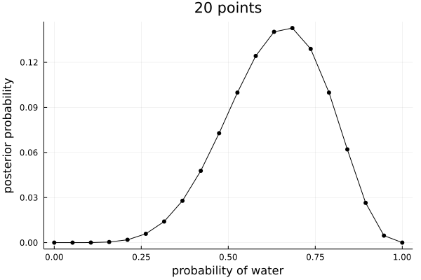
    

    

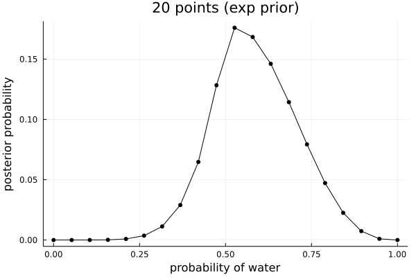
    And with the other two priors suggested:

    step_prior = (x -> if x > .5 1 else 0 end).(p_grid)
    exp_prior = (x -> exp( -5 * abs( x - .5 ) )).(p_grid)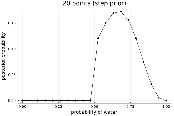
    

    

  • 2.4.4 Quadratic approximation

    I will skip the quadratic approximation example here as there are plenty of proper examples later in the book.

  • 2.4.5 Markov chain Monte Carlo

• 2.5 Summary

• 2.6 Exercises

3. #

Quotes #

More generally, Bayesian golems treat “randomness” as a property of information, not of the world. Nothing in the real world—excepting controversial interpretations of quantum physics—is actually random. Presumably, if we had more information, we could exactly predict everything. We just use randomness to describe our uncertainty in the face of incomplete knowledge.